# Classifying Finnish forest and mire types with Tessera embeddings using tessera-eval
Date: 2026-09-29
Author: Silja Sormunen
Canonical URL: https://geotessera.org/blog/2026-09-29-tessera-eval-finnish-forest-mire
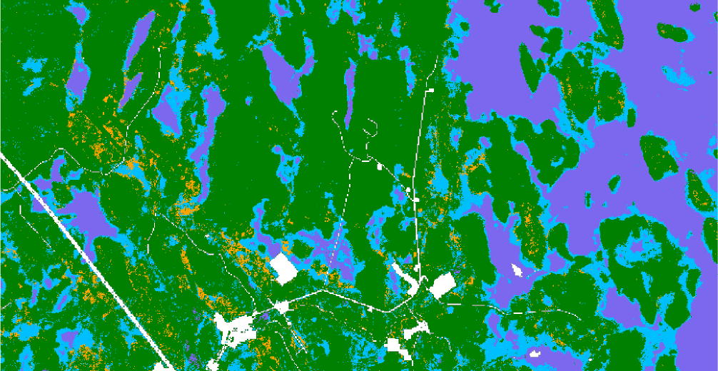
Tessera-eval's predicted site types across the study area near Kemi, northern Finland. Credit: Silja Sormunen / Tessera, University of Cambridge.
*The Python library **tessera-eval**, from the University of Cambridge Tessera team, lets users train a model on Tessera embeddings easily and quickly. In this demonstration, research associate Silja Sormunen uses its command-line tool to find the different types of forest and wetland across a region of northern Finland.*
Geospatial foundation models, like Tessera, compress Earth observation data into rich representations. These representations can be used as input for downstream tasks, such as training a classifier to recognise land-cover or habitat types. However, training and evaluating a classifier from start to finish usually involves several repetitive steps that, while not particularly demanding, can be time-consuming and tedious.
Recently, I built a command-line tool that handles this process for Tessera embeddings, cutting the workflow down to just a few commands. The tool is built around [tessera-eval](https://github.com/ucam-eo/tessera-eval), a Python library for training and evaluating classifiers or regressors on Tessera embeddings, given some labelled ground truth data. Srinivasan Keshav [introduced the library and its Python interface](https://geotessera.org/blog/2026-09-09-evaluating-downstream-tasks-with-tessera-embeddings) in an earlier post. Here, I focus on the command line. The idea is to go from raw embeddings to a working model without needing to write a new Python script: loading embeddings and aligning ground-truth labels onto the embedding grid, then training and evaluating classifiers or regressors using k-fold cross-validation, learning curves, and spatial holdout splits.
In this post, I use this command-line tool to classify types of forest and mire in northern Finland. As ground truth, I use the Finnish multi-source National Forest Inventory data produced by the Natural Resources Institute Finland (Luke), available through the [Paituli spatial data service](https://paituli.csc.fi/download). This data provides maps of several forest and mire variables per pixel, estimated from a combination of field surveys, satellite imagery and other digital georeferenced data. It's good to keep in mind that this data is itself a model output rather than a direct field observation, but I use it for this exploration as it is publicly available. Here, I focus on the coarse site-type classification (the "site main class" variable), which divides forestry land into four categories: mineral soil, pine mire, spruce mire and treeless mire. In what follows, I walk through the process of training a simple site-type classifier from start to finish using only a few commands.
## Loading the data
First, I selected an approximately 10x10 km area in northern Finland near Kemi, where an initial exploratory search showed that the rarest mire type, spruce mire, was less severely underrepresented than the national average. I downloaded Tessera embeddings for this area for 2023 with the command
```bash
tessera-eval load --data ../testing_scripts/luke/vmi/2023/paatyyppi_vmi1x_1923.tif --bbox 24.9,65.79,25.13,65.88 --year 2023 --nodata 32766,32767
```
Here, I gave the area as a bounding box in longitude/latitude degrees and specified that values 32766 and 32767 should be treated as missing/non-forestry data, as noted in the dataset's documentation. This command downloads the Tessera embeddings for the specified area then aligns and resamples the ground-truth raster onto the Tessera 10x10-metre grid. The forest inventory data is already rasterised, so it only needs alignment and resampling. If your ground-truth data consists of labelled polygons in GeoJSON/shapefile format, tessera-eval handles the rasterisation step as well.
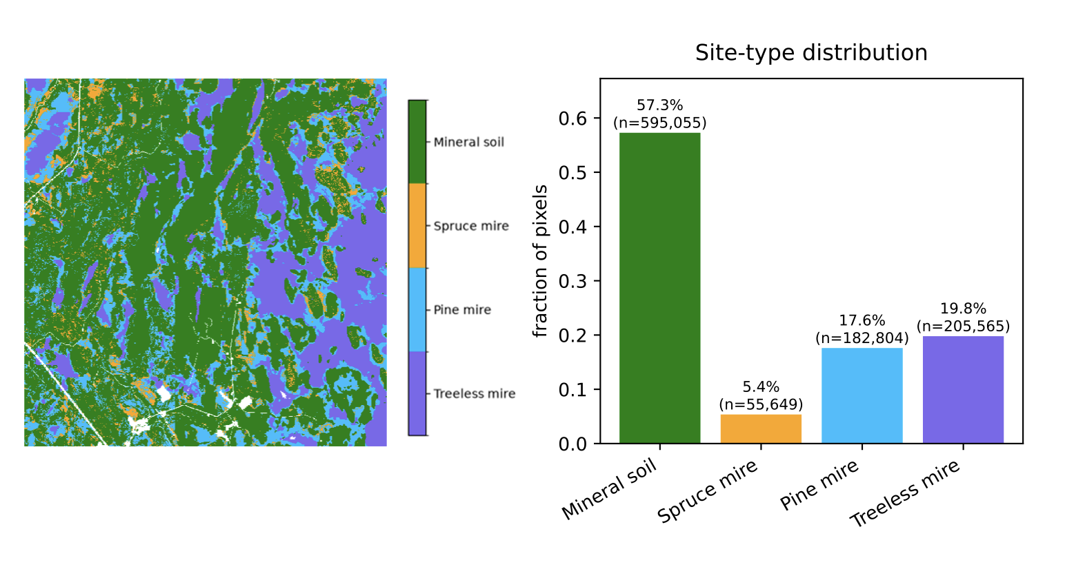
Map of site types in the studied area (left) and the distribution of pixels across classes (right) after resampling.
## Cross-validation on random split
After loading the data, I trained three classifiers, random forest (rf), k-nearest neighbours (nn) and multi-layer perceptron (mlp), to classify site type by running
```bash
tessera-eval kfold --models rf,nn,mlp --k 5 --max-samples 50000 --confusion-matrix
```
This runs 5-fold cross-validation with a random train/test split, capping the training set to 50,000 samples per fold. Multi-layer perceptron performed best in terms of macro-F1 (average macro-F1 0.700, vs 0.619 for rf and 0.667 for nn). Since macro-F1 gives the unweighted mean of per-class F1 scores, poor performance on rare classes pulls the overall score down substantially. This is visible in the automatically printed confusion matrix summary, which shows that recall for the spruce mire class is far lower than for the other three classes, which is unsurprising given that it makes up only about 6% of pixels in this area:
```text
Confusion summary [mlp]:
1.0 (mineral soil): recall 0.92 (most confused with 3.0)
2.0 (spruce mire): recall 0.27 (most confused with 1.0)
3.0 (pine mire): recall 0.63 (most confused with 1.0)
4.0 (treeless mire): recall 0.93 (most confused with 3.0)
```
The full confusion matrix, printed by passing `--confusion-matrix`, shows the absolute predicted counts:
```text
Confusion matrix [mlp] (rows=true, cols=predicted):
1.0 2.0 3.0 4.0
1.0 597,218 16,366 32,552 1,596
2.0 34,927 15,903 8,747 147
3.0 52,044 7,317 124,916 14,335
4.0 1,895 230 15,156 218,865
```
All three classifiers showed a similar pattern: spruce and pine mires were most often confused with mineral soil (for spruce mire, even more often than being classified correctly), while mineral soil was most often confused with pine mire, the second most common mire type in this region.
## How many labels are needed?
Since the embeddings already capture rich information about each pixel's characteristics, the amount of training labels needed is often substantially smaller than with traditional approaches. Next, I explored how the results for multi-layer perceptron change when different percentages of labels are used in training by running
```bash
tessera-eval learning-curve --models mlp --training-pcts 1,5,10,30,50,80
```
The output showed that the performance using only 1% of the labels is already close to the performance with 80% of the labels:
```text
1% [mlp] macro-F1 0.658
5% [mlp] macro-F1 0.674
10% [mlp] macro-F1 0.677
30% [mlp] macro-F1 0.672
50% [mlp] macro-F1 0.667
80% [mlp] macro-F1 0.692
```
This observation is consistent with previous results showing that Tessera performs well already with few labels. Part of the effect can also be explained by how learning-curve samples its training data; rather than drawing pixels completely at random, it aims for an equal number of pixels from every class. At low percentages, this means that even the rarest class (spruce mire) is well represented, as it has enough pixels to supply its equal share. At higher percentages, the rarest class eventually runs out of available pixels and plateaus, while the more common classes keep contributing more. This means that the training set gradually becomes less balanced as the percentage increases, even though the total training size keeps growing.
## Solving the problem of correlated pixels: spatial holdout set
So far I have randomly split the data into train and test sets. However, this approach has a caveat: since neighbouring pixels tend to be highly correlated, a random split places near-identical pixels into train and test sets, so the model isn't really being tested on anything unfamiliar. Because of this, a good performance on the test set may partly reflect how well the model memorises a neighbourhood rather than how well it generalises to truly unseen data.
To truly test the model's ability to generalise, a better approach is to train on one geographic region and test on a separate region. This can easily be done by passing the argument `--spatial-holdout` to the previous command. By default, this splits the area in half by longitude, trains on one half and tests on the other. One can also pass a bounding box for the test set to hold out a specific region.
In my case, treeless mire happens to be much more common in the eastern half of the area than the western half, covering roughly 9% of the west versus 68% of the east. Despite this shift in class frequency, the model still achieved a macro-F1 of 0.60 using only 1% of the training labels and 0.64 using 80% of the labels. To see how much the frequency change itself affects the results, I reran the experiment with a north/south split instead, where the class distributions are much more similar between the two halves. Performance using 80% of the labels rose to 0.682 - a relatively modest difference compared to the east/west split, suggesting that the model has learned features robust to changes in class frequencies.
## Final thoughts
Although there's clearly room to improve and fine-tune the model further, it was nice to see how little effort and how few labels it took to train a classifier that performed solidly even on a spatially separated, class-imbalanced test set. If you'd like to try on your own data, the code for tessera-eval and the command-line interface are available on [GitHub](https://github.com/ucam-eo/tessera-eval). If you prefer working in Python, [Keshav's post](https://geotessera.org/blog/2026-09-09-evaluating-downstream-tasks-with-tessera-embeddings) covers the same steps in code.
---
*[Silja Sormunen](https://geotessera.org/blog/2026-07-11-new-faces-silja-sormunen) is a research associate at the University of Cambridge Department of Computer Science & Technology, where she is exploring new applications for Tessera's embeddings and the information they capture.*